TPC-H Query 1: Performance Optimization Using SQL Server Analysis Services

 

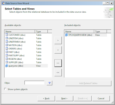
In our previous tutorial, we attempted to reduce the response time for TPC-H Query 1 for scale factor 10. In this tutorial, we will explain how the same query result can be made available using SQL Server Analysis Services to allow end-user to perform multi-dimensional analysis. To begin with, first we will create a view for our TPC-H Query 1 as shown in create view script below:

 
create view TPCHQUERY1VIEW as

SELECT

L_SHIPDATE

, L_RETURNFLAG

, L_LINESTATUS

, SUM(L_QUANTITY) AS SUM_QTY

, SUM(L_EXTENDEDPRICE) AS SUM_BASE_PRICE

, SUM(L_EXTENDEDPRICE*(1-L_DISCOUNT)) AS SUM_DISC_PRICE

, SUM(L_EXTENDEDPRICE*(1-L_DISCOUNT)*(1+L_TAX)) AS SUM_CHARGE

, SUM(L_QUANTITY) AS AVG_QTY_SUM

, SUM(L_EXTENDEDPRICE) AS AVG_PRICE_SUM

, SUM(L_DISCOUNT) AS AVG_DISC_SUM

--, AVG(L_QUANTITY) AS AVG_QTY --We have done AVG_QTY_SUM above

--, AVG(L_EXTENDEDPRICE) AS AVG_PRICE --We have done AVG_PRICE_SUM above

--, AVG(L_DISCOUNT) AS AVG_DISC -- We have done AVG_DISC_SUM

, COUNT_BIG(*) AS COUNT_ORDER

FROM dbo.LINEITEM

--WHERE L_SHIPDATE <= dateadd(dd, -90, cast('1998-12-01' as datetime))

GROUP BY L_SHIPDATE, L_RETURNFLAG, L_LINESTATUS

--ORDER BY L_RETURNFLAG,L_LINESTATUS --invalid in views

go

Once you are done with creating the cube. You can move forward to create Cube using MS SQL Server Analysis Services Project in SQL Server Business Intelligence Studio. For detail on how to create a cube, you can refer to our previous post on this topic at Building Data Cubes: An Introduction to SQL Server Analysis Services. The only difference will be that we will be using the same TPCHQUERY1VIEW  view to create dimensions and cube.

While creating dimension, we will be using the same column as Key Column and Name column.

We will create three dimensions, i.e., L_SHIPDATE, L_RETURNFLAG, and L_LINESTATUS.

We will select all view columns with sum aggregation as measure except the TPCHQUERY1VIEW count. We will not need this for generating TPC-H Query 1 results.

Select all three dimensions that we have created earlier.

Once you are done with CUBE creation and processing. It is not time to view our results. Drag and drop the required dimension and measure in the browse window. TPC-H query extract all records with L_SHIPDATE on or before 1998-09-02. Therefore, we will restrict our result with a filter on L_SHIPDATE dimension.

As you can observe, we do not have any direct provision to calculate AVG_QTY, AVG_PRICE, and AVG_DISC as a measure. Therefore, we will make use of MultiDimensonal eXpressions (MDX) to calculate these three measures. MDX Query below gives us equivalent results as of TPC-H Query 1 using the CUBE that we have just created. We use WITH SET to restrict the records according to L_SHIPDATE dimension. Furthermore, we make use of WITH MEMBER to calculate three averages as required by TPC-H Query 1.

WITH

SET [myset] AS

{[L_SHIPDATE].[L SHIPDATE].&[1992-01-02T00:00:00]:[L_SHIPDATE].[L SHIPDATE].&[1998-09-02T00:00:00]}

MEMBER [Measures].[AVG_QTY] AS

([Measures].[AVG QTY SUM] / [Measures].[COUNT ORDER])

MEMBER [Measures].[AVG_PRICE] AS

([Measures].[AVG PRICE SUM] / [Measures].[COUNT ORDER])

MEMBER [Measures].[AVG_DISC] AS

([Measures].[AVG DISC SUM] / [Measures].[COUNT ORDER])

SELECT

([L_RETURNFLAG].[L RETURNFLAG].members, [L_LINESTATUS].[L LINESTATUS].members) ON ROWS

, 

{

[Measures].[SUM QTY]

, [Measures].[SUM BASE PRICE]

, [Measures].[SUM DISC PRICE]

, [Measures].[SUM CHARGE]

, [Measures].[AVG_QTY]

, [Measures].[AVG_PRICE]

, [Measures].[AVG_DISC]

} ON COLUMNS

FROM

QUERY1CUBE

Snapshot of results from out MDX query are provided in the Figure below.